OVERVIEW

A building structure is typically constructed floor by floor in the case of a reinforced concrete structure or often constructed several floors at a time in the case of a structural steel structure. Even on the same floor, different parts are constructed at different stages.

A typical structural analysis entails applying the loads to the completed structure at once. This results in significant discrepancies as the scale of the building increase, especially as the number of stories increases. Regardless of the type of construction, construction dead loads on a particular floor are typically acting on the structure without the presence of the upper floors during the construction. This actually results in completely different column shortenings from the analysis results based on the “full loading on the completed structure”.  The change of strength gain, creep and shrinkage in the case of reinforced concrete construction compound the discrepancies. MIDAS/Gen enables the engineer to account for the change of geometries and time-dependent material properties during and after the construction.

Each temporary structure at a particular stage of construction affects the subsequent stages. Also, it is not uncommon to install and dismantle temporary supports during construction. The structure constantly changes or evolves as the construction progresses with varying material properties such as modulus of elasticity and compressive strength due to different maturities among contiguous members. The structural behaviors such as deflections and stress re-distribution continue to change during and after the construction due to varying time-dependent properties.

Since the structural configuration continuously changes with different loadings and support conditions, and each construction stage affects the subsequent stages, the design of certain structural components may be even governed during the construction. Without such construction stage analysis, the conventional analysis will not be reliable.

Contents

The procedure used in MIDAS/Gen for carrying out a time-dependent analysis reflecting construction stages is as follows:

1. Create a structural model. Assign elements, loads, and boundary conditions to be activated or deactivated to each construction stage together as a group.
2. Define time-dependent material properties such as creep and shrinkage. The time-dependent material properties can be defined using the standards such as ACI or CEB-FIP, or you may directly define them.
3. Link the defined time-dependent material properties to the general material properties. By doing this, the changes in material properties of the relevant concrete members are automatically calculated.
4. Considering the sequence of the real construction, generate construction stages and time steps.
5. Define construction stages using the element groups, boundary condition groups, and load groups previously defined.
6. Carry out a structural analysis after defining the desired analysis condition.
7. Combine the results of the construction stage analysis and the completed structure analysis.

Analysis Reflecting Erection Sequence

General analysis for a building structure is performed under the assumption that all loads are simultaneously applied to a completed structure. This assumption made every day, however, is not valid in a real construction sequence because a building is constructed by floor-by-floor or lift-by-lift. Even for the same floor, some different parts may be constructed and loaded in different time frames. As a result, true behaviors of a structure may be considerably different from the analysis based on “instantaneous one-time loading” on an “instantaneously constructed structure”. For instance, girders at high floors of a high-rise building may have considerably large moments. Also, we sometimes note inappropriate vertical load distribution to concrete walls, which is relatively higher compared to the distribution to the adjacent frame. Two main reasons can be deduced to contribute to the behaviors:

1. When all loads are simultaneously applied to a completed structure, discrepancies occur due to the applied loads, which are resisted by the upper floor frame that has not yet been constructed.
2. Differential elastic shortenings of vertical members occur when construction dead loads are applied as the construction progresses.

The following describes the discrepancies caused by the first case:

In a real structure, construction dead loads including self-weights at a given floor do not affect the member forces of the upper floors that are yet to be constructed. In the case of a reinforced concrete structure, vertical members followed by a floor are constructed at a given level, and the subsequent floor is erected after the concrete below has been cured for some time. Deformations due to construction dead loads in columns may have taken place considerably at the lower levels. However, in general analyses, the entire structure is subjected to design loads at the same time. In fact, construction dead loads at a particular floor must not be resisted by the upper structure because the upper floors simply do not exist during the construction.

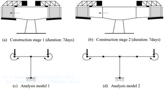
Figure 1 illustrates a 2-story, 2-D plane, concrete frame structure, comparing analysis results between the conventional and erection sequence analyses. The conventional analysis represents the case where the loads are simultaneously applied to the completed structure. Whereas the erection sequence analysis represents the case where separate analysis models are used according to the erection sequence such that the construction loads are applied in two steps to correspond to the models.

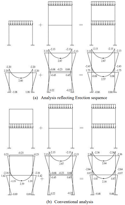
As summarized in Table 1, the erection sequence analysis results show member forces at 90~180% of those obtained from the conventional analysis. In the real construction process, when the construction dead loads are applied to the 1^st stage structure, the member forces of the 1^st stage structure are not affected by the 2^nd stage framing, which is yet to be constructed. In the case of the conventional analysis, however, the non-existing 2^nd stage columns restrain the rotational deformations at the first stage. As a result, the columns of the 1^st and 2^nd stages together sustain the construction loads. This causes discrepancies between the analyses. Therefore, the conventional analysis method may produce considerable discrepancies in design results.

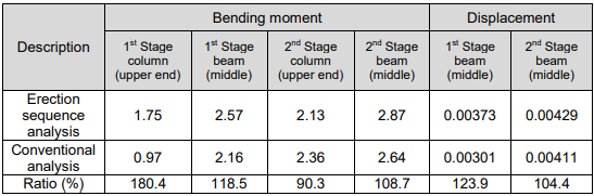
* Ratio =Erection sequence analysis results / Conventional analysis results x 100%

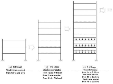
In the case of a structural steel or composite structure, as shown in Figure 2, the steel frame is erected ahead of placing the steel decks and concrete. Accordingly, the first cause for discrepancies may not be of concern for structural steel and composite structures, which are different from concrete buildings in which each floor is completed at a time.

The second cause for discrepancies resulting from the differential shortening of columns is discussed below.

In high-rise concrete buildings, the differential shortening of columns occurs due to elastic shortening, shrinkage and creep under long-term axial loads. The effects of shrinkage and creep on a structure depend on several factors such as concrete strength, construction duration, concrete casting condition, weather condition, etc. In general, the effect of shrinkage is not as extensive as the effects of elastic shortening and creep. It is also very difficult to accurately evaluate the effect of creep in the design phase since creep progresses for a long time and depends on many factors.

In general, columns of a building are designed to be similar in their dimensions for the purpose of maintaining the simplicity of design and serviceability for occupants, despite their tributary areas are not similar to one another. Therefore, differences in tributary areas for columns result in differential shortenings in columns. Differential shortenings may also occur due to unbalanced axial stiffnesses between contiguous members closely spaced such as columns and walls, which have substantially different axial stiffnesses. In concrete structures, changing stiffness during concrete curing can also contribute to differential shortenings. The effect of differential shortening is significant in tall buildings and may produce additional bending moments and shear forces to beam members. This will in turn affect the columns and other members, which are rigidly connected (moment connected) to the beams.

In order to design beam members for gravity loads in a high-rise building, some may have attempted to avoid excessive moments and shear forces by either artificially restraining the vertical movement of columns or increasing the stiffness of columns. This practice may have been carried out with the belief that shortenings are adjusted during the construction. However, the correction virtually achieves nothing structurally. Additional forces resulting from differential shortenings still remain in the members. If differential shortening is ignored member forces can be substantially underestimated, particularly horizontal member forces.

In order to avoid differential shortening, columns must be designed to proportion to their tributary areas. However, this is not always possible for architectural reasons. Figure 3 illustrates a concept of shortening distribution.

For instance, if a unit value is assumed for a concentrated load at each level, story height, modulus of elasticity, and cross-section area of a 5-story column, the relative vertical displacement of each level becomes 1.0. Figure 3 (a) shows a unit load individually applied to the column at each level. The sum of all the displacements is tantamount to the result obtained through conventional analysis. Figure 3 (b) illustrates an erection sequence analysis in which the loads are incrementally applied to individual interim models. A separate analysis is required to calculate the magnitude of vertical length adjustment for “Subsequent” loads such as finish, partition, and cladding. In reinforced concrete building construction, floor levels are generally topped (Up to slab) to the architectural levels at each given floor. However, super-elevating floor levels are often adopted in tall building construction to compensate for subsequent vertical displacements.

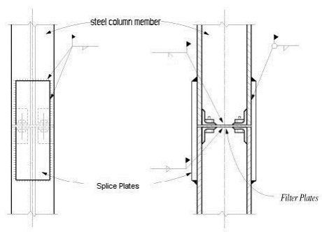
In steel buildings, differential shortening is often compensated by providing filter plates at column splices on site, as shown in Figure 4. Again, the magnitude of compensation will depend on the additional displacements due to subsequent loads.

Elastic axial shortening at floor n, as shown in Figure 3 (c), is given by

• Conventional Analysis:
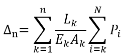
• Erection Sequence Analysis:
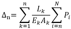
• Displacements due to Loads on the Current and Lower Floors (Up to Slab):
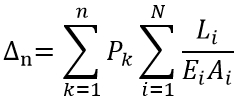
• Displacements due to Loads on the Upper Floors (Subsequent):

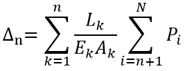
Where,

n = n-th Floor

N = Number of Stories

L_i,k = i-or k-th Floor Story Height

E_i,k = Modulus of Elasticity of Column Located at the i-or k-th Floor

A_i,k = Area of Column Located at the i-or k-th Floor

P_i,k = Construction Load at the i-or k-th Floor

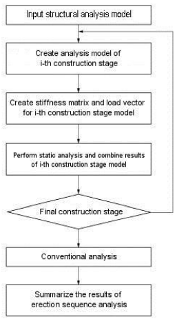
The erection sequence analysis in MIDAS/Gen is developed to analytically overcome the practical problems outlined above, and it reflects the true construction stages of a building structure. Construction dead loads are automatically applied to interim structural models that are formulated to represent each stage of construction and subsequently analyzed. Other loads such as superimposed dead loads, live loads, and lateral loads, which are applied after the completion of the structural frame, are automatically superimposed according to the user-defined load combinations.

MIDAS/Gen separates the model into sub-models for each erection stage and assigns corresponding construction dead loads. The results for each stage are then superimposed to carry out the final erection sequence analysis. Analyses for all remaining loads other than the construction dead loads are carried out on the basis of the conventional analysis. Figure 5 summarizes the analysis steps.

Time-Dependent Material Properties

MIDAS/Gen can reflect time-dependent concrete properties such as creep, shrinkage, and compressive strength gains.

1. Creep and Shrinkage

Creep and shrinkage simultaneously occur in real structures as presented in Figure 6. For practical analysis and design purposes, elastic shortening, creep, and shrinkage are separately considered. The true elastic strain in the figure represents the reduction of elastic strain as a result of concrete strength gains relative to time. In most cases, the apparent elastic strain is considered in analyses. MIDAS/Gen, however, is also capable of reflecting the true elastic strain in analyses considering the time-variant concrete strength gains.

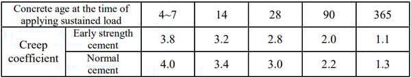
Creep deformation in a member is a function of sustained stress, and a high strength concrete yields less creep deformation relative to a lower strength concrete under identical stress. The magnitudes of creep deformations can be 1.5~3 times those of elastic deformations. About 50% of the total creep deformations take place within the first few months, and the majority of creep deformation occurs in about 5 years.

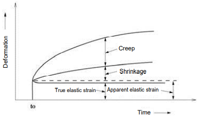Figure 6. Time-Dependent Concrete Deformations

Creep in concrete can vary with the following factors:

1. An increase in water/cement ratio increases creep.
2. Creep decreases with increases in the age and strength of concrete when the concrete is subjected to stress.
3. Creep deformations increase with an increase in ambient temperature and a decrease in humidity.
4. It also depends on many other factors related to the quality of the concrete and conditions of exposure such as the type, amount, and maximum size of aggregate; type of cement; the amount of cement paste; size and shape of the concrete mass; the amount of steel reinforcement; and curing conditions.

Most materials retain the property of creep. However, it is more pronounced in concrete materials, and it contributes to the reduction of pre-stress relative to time. In normal concrete structures, sustained dead loads cause the creep, whereas additional creep occurs in pre-stressed/post-tensioned concrete structures due to the pre-stress effects.

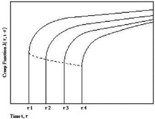
If a unit axial stress σ = 1 exerts on a concrete specimen at the age t₀, the resulting uniaxial strain at the age t is defined as J(t, t₀).

where, J(t, t₀) represents the total strain under the unit stress and is defined as Creep Function.

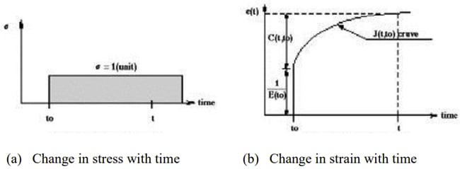
As shown in Figure 7, the creep function J(t, t₀) can be presented by the sum of the initial elastic strain and creep strain as follows:

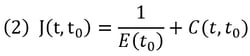
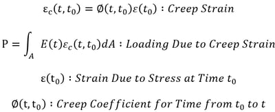
where, E(t₀) represents the modulus of elasticity at the time of the load application, and C(t, t₀) represents the resulting creep deformation at the age t, which is referred to as specific creep. The creep function J(t, t₀) can be also expressed in terms of a ratio relative to the elastic deformation.

where, ø(t, t₀) is defined as the creep coefficient, which represents the ratio of the creep to the elastic deformation. Specific creep can be also expressed as follows:

MIDAS/Gen allows us to specify creep coefficients or shrinkage strains calculated by the equations presented in CEB-FIP, ACI, etc., or we may also directly specify the values obtained from experiments. The user-defined property data can be entered in the form of creep coefficient, creep function, or specific creep.

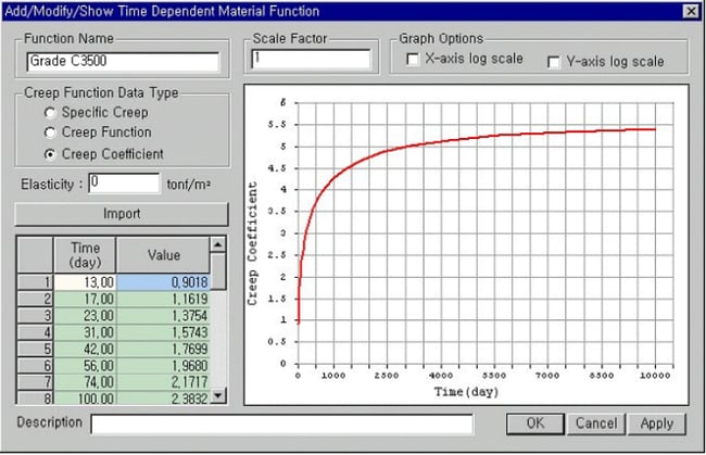
The creep function widely varies with the time of load applications. Due to the concrete strength gains and the progress of hydration with time, the later the loading time, the smaller is elastic and creep strains. Figure 9 illustrates several creep functions varying with time. Accordingly, when the user defines the creep functions, the range of the loading time must include the element ages (loading time) for a time-dependent analysis to reflect the concrete strength gains. For example, if a creep analysis is required for 1000 days for a given load applied to the concrete element after 10 days from the date of concrete placement, the creep function must cover the range of 1010 days. The accuracy of analysis results improves with an increase in the number of creep functions based on different loading times.

Shrinkage is a function of time, which is independent of the stress in the concrete member. Shrinkage strain is generally expressed in time from t₀ to t.

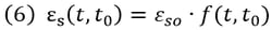
where, ε_so represents the shrinkage coefficient at the final time; f(t, t₀) is a function of time; t stands for the time of observation; t₀  stands for the initial time of shrinkage.

2. Methods of Calculating Creep

Creep is a phenomenon in which deformations occur under sustained loads with time and without necessarily additional loads. As such, a time history of stresses and time become the important factors for determining the creep. Not only does the creep in pre-stressed and post-tensioned concrete members translate into the increase in deformations, but it also affects the pre-stressing in the tendons, thereby affecting the structural behavior. In order to accurately account for time-dependent variables, a time history of stresses in a member and creep coefficients for numerous loading ages are required. Calculating the creep in such a manner demands a considerable amount of calculations and data space. Creep is a non-mechanical deformation, and as such only deformations can occur without accompanying stresses unless constraints are imposed.

One of the general methods used in practice to consider creep in concrete structures is one that a creep coefficient for each element at each stage is directly entered and applied to the accumulated element stress to the present time. Another commonly used method exists whereby specific functions for creep are numerically expressed and integrated relative to stresses and time.

The first method requires creep coefficients for each element for every stage. The second method calculates the creep by integrating the stress time history using the creep coefficients specified in the built-in standards within the program. MIDAS/Gen permits both methods. If both methods are specified for an element, the first method overrides. It is more logical to adopt only one of the methods typically. However, both methods may be used in parallel if a time frame of 20~30 years is selected, or if creep loads are to be considered for specific elements.

If the creep coefficients for individual elements are calculated and entered, the results may vary substantially depending on the coefficient values. For reasonably accurate results, the creep coefficients must be obtained from adequate data on stress time history and loading times. If the creep coefficients at various stages are known from experience and experiments, it can be effective to directly use the values. The creep load group is defined and activated with creep coefficients assigned to elements. The creep loadings are calculated by applying the creep coefficients and the element stresses accumulated to the present.

The user directly enters the creep coefficients and explicitly understands the magnitudes of forces in this method, which is also easy to use. However, it entails the burden of calculating the creep coefficients. The following outlines the calculation method for creep loadings using the creep coefficients.

The following outlines the method in which specific functions of creep are numerically expressed, and stresses are integrated over time. The total creep from a particular time t₀ to a final time t can be expressed as (superposition) integration of a creep due to the stress resulting from each stage.

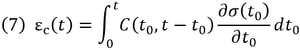
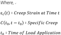
If we assume from the above expression that the stress at each stage is constant, the total creep strain can be simplified as a function of the sum of the strain at each stage as follows:

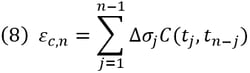
Using the above expression, the incremental creep strain Δε_c,n  between the stages t_n-t_n-1  can be expressed as follows:

If the specific creep is expressed in degenerate kernel (Dirichlet functional summation), the incremental creep strain can be calculated without having to save the entire stress time history.

Using the above specific creep equation, the incremental strain can be rearranged as follows:

(11)

where,

Using the above method, the incremental strain for each element at each stage can be obtained from the resulting stress from the immediately preceding stage and the modified stress accumulated to the previous stage. This method provides relatively accurate analyses reflecting the change in stresses. Once we enter necessary material properties without separately calculating creep coefficients, the program automatically calculates the creep. Despite the advantage of easy application, it shares some disadvantages; since it follows the equations presented in Standards, it restricts us to input specific creep values for specific elements.

This method is greatly affected by the analysis time interval. Time intervals for construction stages in general cases are relatively short and hence do not present problems. However, if a long time interval is specified for a stage, it is necessary to internally divide into sub-time intervals to closely reflect the creep effects. Knowing the characteristics of creep, the time intervals should be preferably divided into a log scale.

MIDAS/Gen is capable of automatically dividing the intervals into the log scale based on the number of intervals specified by the user. There is no fast rule for an appropriate number of time intervals. However, the closer the division, the closer to the true creep can be obtained. In the case of a long construction stage interval, it may be necessary to divide the stage into a number of time steps.

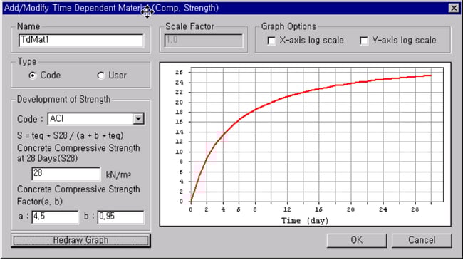
3. Development of Concrete Compressive Strength

MIDAS/Gen reflects the changes in concrete compressive strength gains relative to the maturities of concrete members in analyses. The compressive strength gain functions can be defined as per standard specifications such as ACI and CEB-FIP as shown in Figure 10, or the user is free to define one directly. MIDAS/Gen thus refers to the concrete compressive strength gain curves, and it automatically calculates the strengths corresponding to the times defined in the construction stages and uses them in the analysis.

The time-dependent material properties (creep, shrinkage, and concrete compressive strength gain) defined in Figure 10 can be applied in analyses in conjunction with conventional material properties. This linking process is simply necessary for the program’s internal data structure.

Input Process of Time-Dependent Material Properties

Time-dependent material properties of elements reflecting their maturities are required for the construction stage and heat of hydration analyses in which MIDAS/Gen accounts for creep and shrinkage of concrete. Observe the following steps for entering time-dependent material properties:

1. Define the material properties related to creep and shrinkage in Model > Properties > Time Dependent Material (Creep/Shrinkage)
2. 

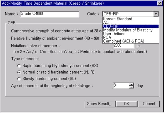
In order to select User Defined in the Code field, first define the creep and shrinkage functions in Model > Properties > Time Dependent Material (Creep/Shrinkage) Function.

1. Define the time variant modulus of elasticity in Model > Properties > Time Dependent Material (Comp. Strength)
2. 
   

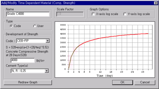
   Figure 12. Change of Modulus of Elasticity of Concrete

1. Link the time dependent material properties to the general material properties already entered in Model > Properties > Time Dependent Material Link
   
   

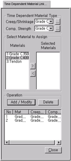
   Figure 13. Time Dependent Material Link Dialog Bar

Definition and Composition of Construction Stages

MIDAS/Gen allows us to specify construction stages and their compositions in detail to reflect the true erection sequence of construction. This is an extremely powerful tool, which can be applied to various construction stage analyses related to different erection methods practiced in building construction.

MIDAS/Gen defines the three distinct stages, which retain the following characteristics:

• Base Stage
  

  When the construction stage is undefined, a general analysis may be performed. If the construction stage is defined, the analysis is disabled; the structural modeling is completed; and the element, boundary and load groups are defined and composed.

• Construction Stage
  

  Structural analyses are actually carried out for the construction stages. For each construction stage, relevant element, boundary and load groups are activated.

• Post-Construction Stage

  Being the post-construction stage of the construction, analyses are carried out for the construction stage loads as well as other general loads, response spectrum, etc.   

Each construction stage is composed of activated (or deactivated) element, boundary and load groups. By the combination of the three groups with each group defined by the process of activation and deactivation, tremendous flexibility exists in composing the stages.

The following are the contents included in each construction stage:

1. Activation (creation) and deactivation (deletion) of elements with certain maturities (ages)
2. Activation and deactivation of loadings at certain points in time
3. Changes in boundary conditions

The concept of construction stages used in MIDAS/Gen is illustrated in Figure 14. Construction stages can be readily defined by duration for each stage. A construction stage with ‘0’ duration is possible, and the first and last steps are basically created once a construction stage is defined. Activation and deactivation of elements, boundary conditions and loadings are practically accomplished at each step.

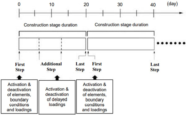
Activation and deactivation of changing conditions such as new and deleted elements, boundary conditions, and loadings basically take place at the first step of each construction stage. Accordingly, construction stages are created to reflect the changes of structural systems that exist in real construction relative to the construction schedule. That is, the number of construction stages increases with the increase in the number of temporary structural systems.

Structural system changes in terms of active elements and boundary conditions are defined only at the first step of each construction stage. However, additional steps can be defined within a given construction stage for ease of analysis to reflect loading changes. This allows us to specify delayed loadings representing, for instance, temporary construction loads while maintaining the same geometry without creating additional construction stages.

If many additional steps are defined in a construction stage, the accuracy of analysis results will improve since the time dependent analysis closely reflects creep, shrinkage and compressive strengths. However, if too many steps are defined, the analysis time may be excessive, thereby compromising efficiency. Moreover, if time dependent properties (creep, shrinkage and modulus of elasticity) are not selected to participate in Analysis>Construction Stage Analysis Control Data and the analysis is subsequently carried out, the analysis results do not change regardless of the number of steps defined.

Subsequent to activating certain elements with specific maturities in a construction stage, the maturities continue with the passage of subsequent construction stages. The material properties of the elements in a particular construction stage change with time. MIDAS/Gen automatically calculates the properties by using only the elements’ maturities based on the pre-defined time dependent material properties (Model>Properties>Time Dependent Material). We are not required to define the changing material properties at every construction stage.

If two elements are activated with an identical maturity in an identical construction stage, the elapsed times for both elements are always identical. However, there are occasions where only selective elements are required to pass the time among the elements activated at the same time. This aging of selective elements is accomplished by using the time load function (Load>Time Loads for Construction Stage).

When specific elements are activated in a construction stage, the corresponding maturities must be assigned to the elements. Creating elements with ‘0’ maturity represents the instant when the fresh concrete is cast. However, a structural analysis model does not typically include temporary structures such as formwork/falsework, and as such unexpected analysis results may be produced if the analysis model includes immature concrete elements.

Especially, if elements of ‘0’ maturity are activated, and an analysis is carried out reflecting the time dependent compressive strength gains, significantly meaningless displacements may result due to the fact that no concrete strength can be expected in the first 24 hours of casting. A correct method of modeling a structure for considering construction stages may be that the wet concrete in and with the formwork is considered as loading in the temporary structure, and that the activation of the concrete elements is assumed after a period of time upon removal of the formwork/falsework.

If new elements are activated in a particular construction stage, the total displacements or stresses accumulated up to the immediately preceding construction stage do not affect the new elements. That is, the new elements are activated with ‘0’ internal stresses regardless of the loadings applied to the current structure.

When elements are deactivated, and 100% stress redistribution is assigned, all the internal stresses in the deactivated elements are redistributed to the remaining structure, and the internal stresses of the elements constituting the remaining structure will change. This represents loading equal and opposite internal forces at the boundaries of the removed elements. On the other hand, if 0% stress redistribution is assigned, the internal stresses of the deactivated elements are not transferred to the remaining structure at all, and the stresses in the remaining elements thus remain unchanged. The amount of the stresses to be transferred to the remaining elements can be adjusted by appropriately controlling the rate of stress redistribution. This flexible feature can be applied to consider the incomplete or partial transfer of the stresses in the deactivated elements in a construction stage analysis.

A typical example can be a tunnel analysis application. In a tunnel construction stage analysis, the elements in the part being excavated do not relieve the stresses to the remaining support structure all at once. The use of rock bolts or temporary supports may transfer the internal stresses of the deactivated (excavated) elements gradually to the remaining structures of subsequent construction stages. Accordingly, the internal stresses of deactivated elements can be gradually distributed to the interim structures over a number of construction stages.

If “original” is selected while a boundary condition is activated, the boundary condition is activated at the original (undeformed) node location. This is achieved internally by applying a forced displacement to the node in the direction opposite to the displacement of the immediately preceding construction stage. Additional internal stresses resulting from the forced displacement will be accounted for in the structure. Conversely, if the option “deformed” is selected, the node for which the boundary condition is to be activated will be located at the deformed location as opposed to the original location.

In a time dependent analysis reflecting construction stages, the structural system changes and loading history of the previous stages affect the analysis results of the subsequent stages. MIDAS/Gen thus adopts the concept of accumulation. Rather than performing analyses for individual structural models pertaining to all the construction stages, incremental structural and loading changes are entered and analyzed for each construction stage. The results of the current stage are then added to that of the preceding stage.

If loading is applied in a construction stage, the loading remains effective in all the subsequent construction stages unless it is deliberately removed. Elements are similarly activated for a given construction stage. Only the elements pertaining to the relevant construction stage are activated as opposed to activating all the necessary elements for the stage. Once-activated elements cannot be activated again, and only those elements can be deactivated.

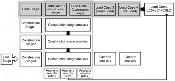
The loading cases to be applied in a construction stage analysis must be defined as the “construction stage load” type. Even if a number of loading cases exist in a construction stage analysis, their results are combined as a single result as depicted in Figure 16. This is because the nonlinearity of time dependent material properties in a construction stage analysis renders a linear combination of load cases impossible. A construction stage analysis produces accumulated analysis results and the maximum/minimum values as shown in Figure 16. The results of the construction stage analysis thus obtained can be now combined with the results of the conventional load cases.

We often encounter occasions where intermediary construction stages are structurally significant enough to warrant full investigation. Some special loadings perhaps related to construction activities can be engaged in the analysis. MIDAS/Gen allows us to specify the “post-construction stage” to an intermediate stage, which can be analyzed as if it was the final completed structure. Once a structure pertaining to a construction stage is designated as the “post-construction stage”, all general load cases can be applied, and various analyses such as time history and response spectrum can be carried out.

Procedure for Construction Stage Analysis

A typical modeling procedure for construction stage analysis is as follows:

1. Model the complete structure except for the boundary and load conditions.
2. Define the element groups in Model > Group > Define Structure Group Assign the elements that will be activated (constructed) and deactivated (dismantled) at the same time to the defined element groups.
3. Define the boundary groups in Model > Group > Define Boundary Group
4. Define the load groups in Model > Group > Define Load Group
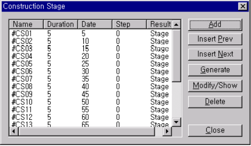
5. Compose the construction stages by clicking the “Add” button in Load > Construction Stage Analysis Data > Define Construction Stage. You may click the “Generate” button to define a number of construction stages of equal duration followed by clicking the Modify/Show button to compose each construction stage.
6. 
   
   

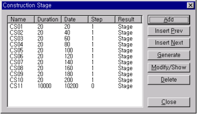
   Figure 17. Define Construction Stage Dialog Box

7. In the Compose Construction Stage dialog box, enter the duration of the construction stage and select whether or not to save the analysis results. If loadings are applied with time intervals to the same structural system within the same construction stage, Additional Steps corresponding to the loading times may be defined.
8. 
   

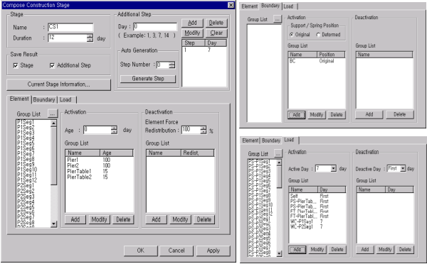
Figure 18. Compose Construction Stage Dialog Box

1. Activate and/or deactivate relevant element groups selected from the Group List under the Element tab. The Age represents the maturity at the start of the stage. The Element Force Redistribution represents the distribution of the internal forces of the elements being deactivated.
2. Activate and/or deactivate relevant boundary groups selected from the Group List under the Boundary tab.
3. Activate and/or deactivate relevant load groups selected from the Group List under the Load tab. The Active Day and Inactive Day represent the timing of load application and removal respectively.
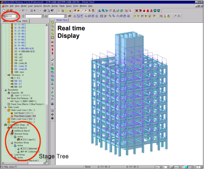
4. Upon completion of composing construction stages, move around the construction stages in Stage Toolbar to enter the boundary and load conditions corresponding to the boundary and load groups of each construction stage.

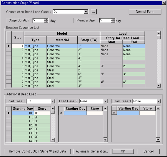
The above outlines the modeling procedure whereby the user directly defines the construction stages individually. We may also automatically generate all the data necessary for the construction stage analysis using Load > Construction Stage Analysis Data > Construction Stage Wizard for Building Structure. Changes can be made subsequently in Compose Construction Stage.