OVERVIEW

Boundary conditions represent the status of connections between the structure and neighboring structures such as foundations. Boundary conditions are distinguished by nodal boundary conditions and element boundary conditions.

Nodal boundary conditions:

The constraint for the degree of freedom
Elastic boundary element (Spring support)
Elastic link element (Elastic Link)

Element boundary conditions:

Element end release
Rigid end offset distance (Beam End Offset)
Rigid link

The constraint function may be used to constrain specific nodal displacements or connecting nodes among elements such as truss, plane stress, and plate elements, where certain degrees of freedom are deficient.

^* Refer to “Model > Boundaries > Supports” of Online Manual.

Nodal constraints are applicable for 6 degrees of freedom with respect to the Global Coordinate System (GCS) or the Node local Coordinate System (NCS).

Figure 1 illustrates a method of specifying constraints on the degrees of freedom of a planar frame model. Since this is a two-dimensional model with permitted degrees of freedom in the GCS X-Z plane, the displacement d.o.f. in the GCS X-direction and the rotational d.o.f. about the GCS X and Z axes need to be restrained at all the nodes, using Model>Boundaries>Supports.

For node N1, which is fixed support, the Supports function is used to additionally restrain the displacement d.o.f. in the GCS X and Z-directions and the rotational d.o.f. about the GCS Y-axis.

* Use the function “Model > Structure Type” for convenience when analyzing two-dimensional problems.

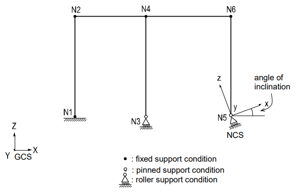
For node N3, which is roller support, the displacement d.o.f. in the GCS Z direction is additionally restrained.

For node N5, which is roller support in an NCS, the NCS is defined first at an angle to the GCS X-axis. Then the corresponding displacement degrees of freedom are restrained in the NCS using Supports.

^* Refer to “Model > Boundaries > Node Local Axis” of Online Manual.

Nodal constraints are assigned to supports where displacements are truly negligible. When nodal constraints are assigned to a node, the corresponding reactions are produced at the node. Reactions at nodes are produced in the GCS, or they may be produced in the NCS if defined.

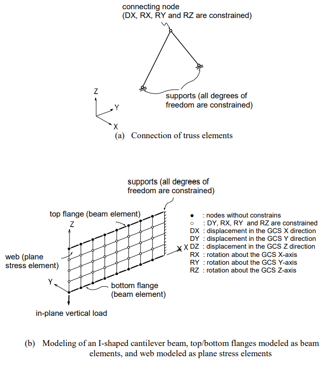
Figure 2 shows examples of constraining deficient degrees of freedom of elements using Supports.

In Figure 2 (a), the displacement d.o.f. in the X-axis direction and the rotational d.o.f. about all the axes at the connecting node are constrained because the truss elements have the axial d.o.f. only.

Figure 2 (b) represents an I-beam where the top and bottom flanges are modeled as beam elements and the web is modeled with plane stress elements. The beam elements have 6 d.o.f. at each node, and as such where the plane stress elements are connected to the beam elements, no additional nodal constraints are required. Whereas, the out-of-plane displacement d.o.f. in the Y direction and the rotational d.o.f. in all directions are constrained at the nodes where the plane stress elements are connected to one another. Plane stress elements retain the in-plane displacement degrees of freedom only.

Elastic Boundary Elements (Spring Supports)

Elastic boundary elements are used to define the stiffness of adjoining structures or foundations. They are also used to prevent singular errors from occurring at the connecting nodes of elements with limited degrees of freedom, such as truss, plane stress, plate element, etc.

* Refer to “Model > Boundaries > Point Spring Supports” of Online Manual.

Spring supports at a node can be expressed in six degrees of freedom, three translational, and three rotational components with respect to the Global Coordinate System (GCS). The translational and rotational spring components are represented in terms of unit force per unit length and unit moment per unit radian respectively.

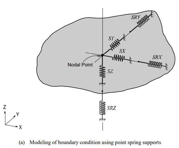
Spring supports are readily applied to reflect the stiffness of columns, piles, or soil conditions. When modeling sub-soils for foundation supports, the modulus of subgrade reaction is multiplied by the tributary areas of the corresponding nodes. In this case, it is cautioned that soils can resist compressions only.

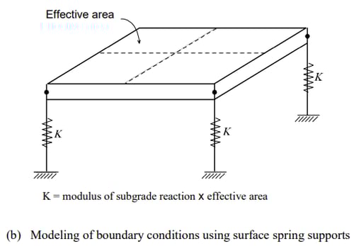
MIDAS/Gen provides Surface Spring Supports to readily model the boundary conditions of the subsurface interface. The Point Spring is selected in Model>Boundaries>Surface Spring Supports and the modulus of subgrade reaction is specified in each direction. The soil property is then applied to the effective areas of individual nodes to produce the nodal spring stiffness as a boundary condition. In order to reflect the true soil characteristics, which can sustain compression only, Elastic Link (compression-only) is selected and the modulus of subgrade reaction is entered for the boundary condition.

* Refer to “Model > Boundaries > Surface Spring Supports” of Online Manual.

Table 1 summarizes moduli of subgrade reaction for soils that could be typically encountered in practice. It is recommended that both maximum and minimum values be used separately, and conservative values with discretion are adopted for design.

The axial stiffness of spring supports for columns or piles can be calculated by EA/H, where E is the modulus of elasticity for columns or piles, A is the Effective Cross-Sectional Area, and H is Effective Length.

Table 1. Typical Values of Moduli of Subgrade Reaction for Soils 

(Reference. “Foundation Analysis and Design” by Joseph E. Bowles 4th Edition)

Rotational spring components are used to represent the rotational stiffness of contiguous boundaries of the structure in question. If the contiguous boundaries are columns, the stiffness is calculated by αEI/H, where α is a rotational stiffness coefficient, I is Effective Moment of Inertia, and H is Effective Length.

Generally, boundary springs at a node are entered in the direction of each d.o.f. For more accurate analyses, however, additional coupled stiffness associated with other degrees of freedom needs to be considered. That is, springs representing coupled stiffness may become necessary to reflect rotational displacements accompanied by translational displacements. For instance, it may be necessary to model a pile foundation as boundary spring supports. A more rigorous analysis could be performed by introducing coupled rotational stiffness in addition to the translational stiffness in each direction.

^* Refer to “Model > Boundaries > General Spring Supports” of Online Manual.

Boundary springs specified at a node, in general, follow the GCS unless an NCS is specified, in which case they are defined relative to the NCS.

Singular errors are likely to occur when stiffness components in certain degrees of freedom are deficient subsequent to formulating the stiffness. If the rotational stiffness components are required to avoid such singular errors, it is recommended that the values from 0.0001 to 0.01 be used. The range of the values may vary somewhat depending on the unit system used. To avoid such singular errors, MIDAS/Gen thus provides a function that automatically assigns stiffness values, which are insignificant to affect the analysis results.

* Refer to “Analysis > Main Control Data” of Online Manual.

Elastic Link Element

An elastic link element connects two nodes to act as an element, and the user defines its stiffness. Truss or beam elements may represent elastic links.

However, they are not suitable for providing the required stiffness with the magnitudes and directions that the user desires. An elastic link element is composed of three translational and three rotational stiffnesses expressed in the ECS.

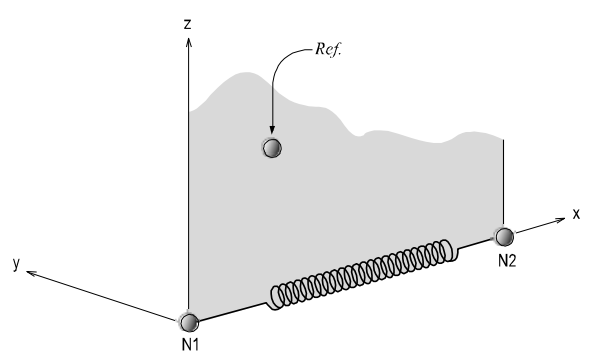
The translational and rotational stiffnesses of an elastic link element are expressed in terms of unit force per unit length and unit moment per unit radian respectively. Figure 4 presents the directions of the ECS axes. An elastic link element may become a tension-only or compression-only element, in which case the only directional stiffness can be specified is in the ECS x-axis.

Examples for elastic link elements include elastic bearings of a bridge structure, which separate the bridge deck from the piers. Compression-only elastic link elements can be used to model the soil boundary conditions. The rigid link option connects two nodes with an “infinite” stiffness.

* Refer to “Model> Boundaries > Elastic Link” of Online Manual.

General Link Element

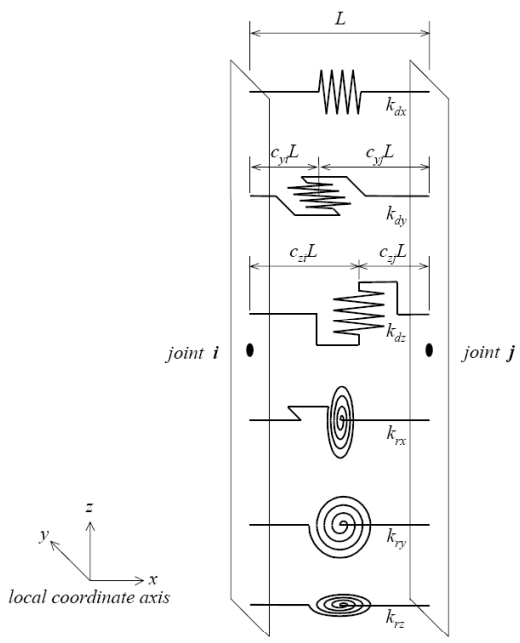
The General Link element is used to model dampers, base isolators, compression-only element, tension-only element, plastic hinges, soil springs, etc. The 6 springs individually represent 1 axial deformation spring, 2 shear deformation springs, 1 torsional deformation spring, and 2 bending deformation springs as per Figure 5. Among the 6 springs, only selective springs may be partially used, and linear and nonlinear properties can be assigned. The general link can be thus used as linear and nonlinear elements.

The General Link element can be largely classified into Element type and Force type depending on the method of applying it to analysis. The Element type general link element directly reflects the nonlinear behavior of the element by renewing the element stiffness matrix. The Force type, on the other hand, does not renew the stiffness matrix, but rather reflects the nonlinearity indirectly by converting the member forces calculated based on the nonlinear properties into external forces.

First, the Element type general link element provides three types, Spring, Dashpot and Spring, and Dashpot. The Spring retains linear elastic stiffness for each of 6 components, and the Dashpot retains linear viscous damping for each of 6 components.

The Spring and Dashpot is a type, which combines Spring and Dashpot. All of the three types are analyzed as linear elements. However, the Spring type general link element can be assigned inelastic hinge properties and used as a nonlinear element. This can be mainly used to model plastic hinges, which exist in parts in a structure or nonlinearity of soils. However, this can be used as a nonlinear element only in the process of nonlinear time history analysis by direct integration. Also, viscous damping is reflected in linear and nonlinear time history analyses only if “Group Damping” is selected for damping for the structure.

The Force type general link element can be used for dampers such as Viscoelastic Damper and Hysteretic System, seismic isolators such as Lead Rubber Bearing Isolator and Friction Pendulum System Isolator, Gap (compression-only element), and Hook (tension-only element). Each of the components retains effective stiffness and effective damping. You may specify nonlinear properties for selective components.

The Force type general link element is applied in the analysis as below. First, it is analyzed as a linear element based on the effective stiffness while ignoring the effective damping in static and response spectrum analyses. In linear time history analysis, it is analyzed as a linear element based on the effective stiffness, and the effective damping is considered only when the damping selection is set as “Group Damping”. In nonlinear time history analysis, the effective stiffness acts as virtual linear stiffness, and as indicated before, the stiffness matrix does not become renewed even if it has nonlinear properties.

Also, because the nonlinear properties of the elements are considered in the analysis, effective damping is not used. This is because the role of effective damping indirectly reflects energy dissipation due to the nonlinear behavior of the Force type general link element in linear analysis. The rules for applying the general link element noted above are summarized in Table 2.

When the damping selection is set as “Group Damping”, the damping of the element type general link element and the effective damping of the force type general link element are reflected in the analysis as below. First, when linear and nonlinear analyses are carried out based on modal superposition, they are reflected in the analyses through modal damping ratios based on strain energy.

On the other hand, when linear and nonlinear analyses are carried out by direct integration, they are reflected through formulating the element damping matrix.

If element stiffness or element-mass-proportional damping is specified for the general link element, the analysis is carried out by adding the damping or effective damping specified for the properties of the general link element.

<Table 2> Rules for Applying General Link Element

(Reference. Damping and effective Damping are considered only when the damping option is set to “Group Damping”.)

The locations of the 2 shear springs may be separately specified on the member. The locations are defined in ratios by the distances from the first node relative to the total length of the member. If the locations of the shear springs are specified and shear forces are acting on the nonlinear link element, the bending moments at the ends of the member are different. The rotational deformations also vary depending on the locations of the shear springs. Conversely, if the locations of the shear springs are unspecified, the end bending moments always remain equal regardless of the presence of shear forces.

The degrees of freedom for each element are composed of 3 translational displacement components and 3 rotational displacement components regardless of the element or global coordinate system. The element coordinate system follows the convention of the truss element. Internal forces produced for each node of the elements consist of 1 axial force, 2 shear forces, 1 torsional moment, and 2 bending moments. The sign convention is identical to that of the beam element. In calculating the nodal forces of the element, the nodal forces due to damping or effective damping of the general link element are found based on Table2. However, the nodal forces due to the element mass or element stiffness-proportional damping are ignored.

Element End Release

When two elements are connected at a node, the stiffness relative to the degrees of freedom of the two elements is reflected. Element End Release can release such stiffness connections. This function can be applied to beam and plate elements, and the methods of which are outlined below.

Beam End Release is applicable for all the degrees of freedom of the two nodes of an element. Using partial fixity coefficients can create partial stiffness of elements. If all three rotational degrees of freedom are released at both ends of a beam element, then the element will behave like a truss element.

* Refer to “Model > Boundaries > Beam End Release” of Online Manual.

Similarly, Plate End Release is applicable for all the degrees of freedom of three or four nodes constituting a plate element. Note that the plate element does not retain the rotational degree of freedom about the axis normal to the plane of the element. If all the out-of-plane rotational d.o.f. are released at the nodes of a plate element, this element then behaves like a plane stress element.

* Refer to “Model> Boundaries > Plate End Release” of Online Manual.

The end releases are always specified in the Element Coordinate System (ECS). Cautions should be exercised when stiffness in the GCS is to be released. Further, the change in stiffness due to end releases could produce singular errors, and as such the user is encouraged to specify end releases carefully through a comprehensive understanding of the entire structure.

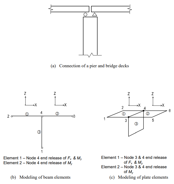
Figure 6 shows boundary condition models depicting the connections between a pier and bridge decks, using end releases for beam and plate elements.

Rigid End Offset Distance

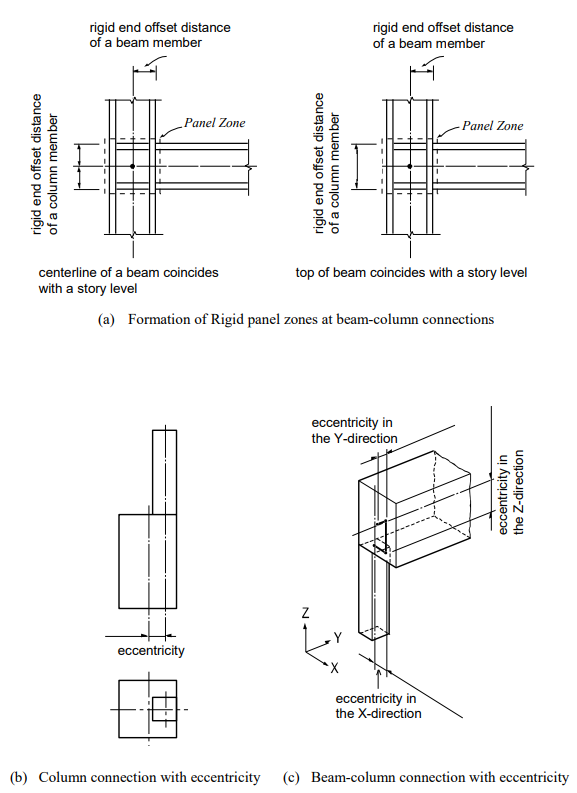
Frame members of civil and building structures are typically represented by element centerlines. Whereas, physical joint sizes (panel zones) actually do exist at the intersections of the element centerlines. Ignoring such panel zones in the analysis will result in larger displacements and moments. In order to account for element end eccentricities and panel zone effects at beam-column connections, MIDAS/Gen provides the following two methods: Note that the terms, beams, and girders are interchangeably used in this section. (See Figure 7)

1. MIDAS/Gen automatically calculates rigid end offset distances for all panel zones where column and beam members intersect.

* Refer to “Model > Boundaries>Panel Zone Effects” of Online Manual.

2. The user directly defines the rigid end offset distances at beam-ends.

* Refer to “Model > Boundaries > Beam End Offsets” of Online Manual.

Rigid end offset distances are applicable only to beam elements, including tapered beam elements, in MIDAS/Gen.

Automatic consideration of panel zone stiffness

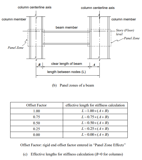
If the bending and shear deformations in the panel zones are ignored, the effective length for member stiffness can be written as:

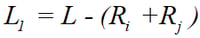
where, L is the length between the end nodes, and R_i and R_j are the rigid end offset distances at both ends. If the element length is simply taken as L₁, the result will contain some errors by ignoring the actual rigid end deformations. MIDAS/Gen, therefore, allows the user to alleviate such errors by introducing compensating factors for rigid end offset distances (Offset Factors).

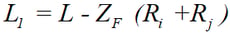
where, Z_F is an offset factor for rigid end offset distance.

The value of the offset factor for rigid end offset distance varies from 0 to 1.0. The user’s discretion is required for determining the factor as it depends on the shapes of connections and the use of reinforcement.

The rigid end offset factor does not affect the calculation of axial and torsional deformations. The entire element length (L) is used for such purposes.

Using Model>Boundaries>Panel Zone Effects in MIDAS/Gen, the GCS Z-axis is automatically established opposite to the gravity direction, and the rigid end offset distances of the panel zones are automatically considered. Note that the rigid end offset distances are applicable only to the beam-column connections. The columns represent the elements parallel to the GCS Z-axis, and the beams represent the elements parallel to the GCS X-Y plane.

* Refer to “Model > Structure Type” of Online Manual.

When the Panel Zone Effects function is used to calculate the rigid end offset distances automatically, the user may select the “Offset Position” for the “Output Position”. In that case, the element stiffness, applications of self-weight and distributed loads, and the output locations of member forces vary with the offset locations adjusted by the offset factor. If “Panel Zone” is selected, the offset factor is reflected in the element lengths for the element stiffness only. The locations for applying self-weight and distributed loads and the output locations of member forces are determined on the basis of the boundaries of the panel zones, i.e., column faces for beams and beam faces for columns.

Selecting “Offset Position” with an offset factor, 1.0 for “Output Position” in Panel Zone Effects is tantamount to selecting “Panel Zone” with an offset factor of 1.0. Conversely, selecting “Offset Position” with an offset factor of 0.0 for “Output Position” becomes equivalent to a case where no rigid end offset distances are considered.

When rigid end offset distances are to be automatically calculated by using Panel Zone Effects, “Output Position” determines the way in which self-weight and distributed loads are applied and the output locations of member forces.

▶Element stiffness calculation

In calculating the axial and torsional stiffnesses of an element, the distance between the end nodes is used. Whereas, an adjusted length, L₁=L-Z_F (R_i+R_j), which reflects the offset factor, is used for the calculation of the shear and bending stiffnesses, regardless of the selection of the location for member force output (See Figure 8).

▶Calculation of distributed loads

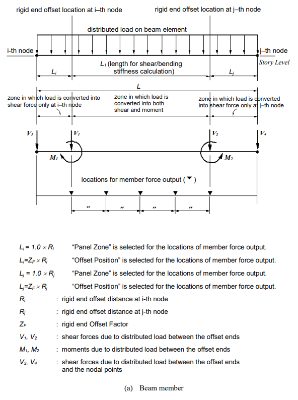
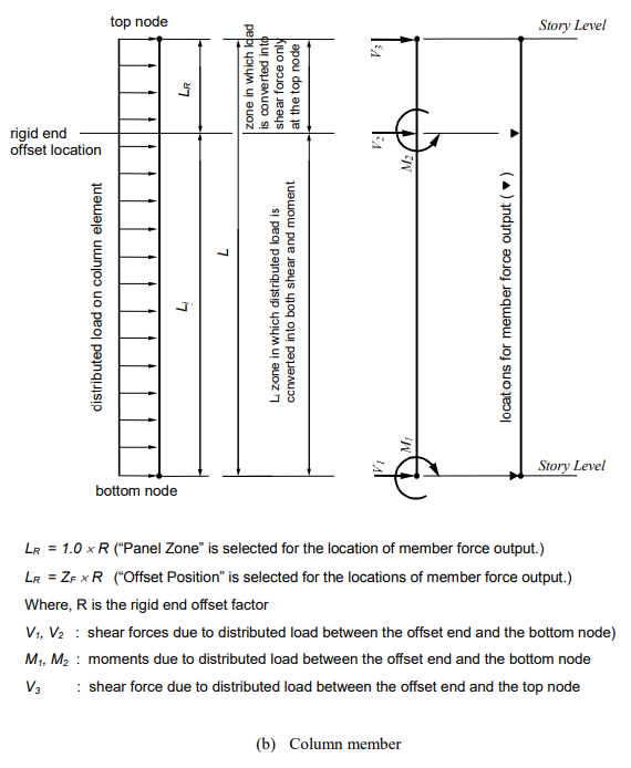
If “Panel Zone” is selected for “Output Position”, any distributed load within a rigid end offset distance is transferred to the corresponding node. The remaining distributed loads are converted to shear forces and moments as shown in Figure 9. If “Offset Position” is selected for “Output Position”, the above forces are calculated relative to the rigid end offset locations that reflect the offset factor.

▶Length considered for the self-weight

The self-weight of a column member is calculated for the full element length without the effect of rigid end offset distances. For the self-weight of a beam, the full nodal distance less the rigid end offset distances, L₁=L-(R_i+R_j), is used when “Panel Zone” is selected for “Output Position”. If “Offset Position” is selected for “Output Position”, the full nodal distance is reduced by the adjusted rigid end offset distances, L₁=L-Z_F (R_i+R_j). The self-weight calculated in this manner is converted into shear forces and moments using the load calculation method described above. 

▶Output position of member forces

If “Panel Zone” is selected for “Output Position”, the member forces for columns and beams are produced at the ends of the panel zones and the quarter points of the net lengths between the panel zones. If “Offset Position” is selected for “Output Position” in the case of beams, the results are produced at similar positions relative to the adjusted rigid end offset distances. Note that the output positions for the “Panel Zone” are identical to the case where “Offset Position” is selected for “Output Position” with an offset factor of 1.0.

▶Rigid end offset distance when the beam end release is considered

If one or both ends of a column or a beam are released to form pinned connections, the rigid end offset distances for the corresponding nodes will not be considered.

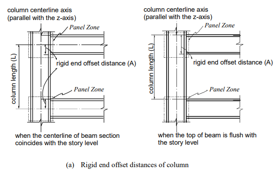
▶Calculation of rigid end offset distances in column members

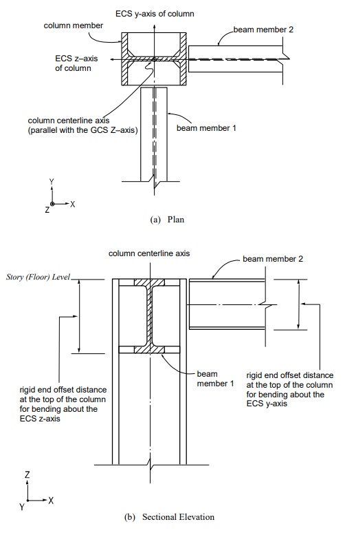
The full length of a column member is taken as a story-height between adjoining floors. In calculating the length, two assumptions are made in MIDAS/Gen; (1) the centerlines of beam sections coincide with the story level line, and (2) the tops of beam sections are flush with the story level line. The rigid end offset distances of columns vary with the two assumptions. If the first assumption is made, the end offsets are calculated at both top and bottom ends of the columns. Meanwhile, with the second assumption, the end offsets are considered only at the tops of the columns (See Figure 8).

* Refer to “Align Top of Beam Section to Floor (X-Y Plane) for Panel Zone Effect/Display in Model > Structure Type”.

At a connection point of a column member and beam (girder) members, the rigid end offset distances of the column is calculated on the basis of the depths and directions of the connected beams. In the case of a beam-column connection as shown in Figure 10, the rigid end offset distances of the column are calculated separately for the ECS y and z-axes.

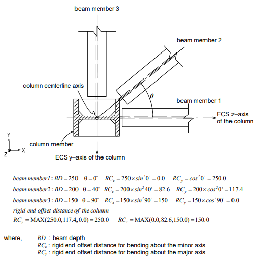
When multi-directional beam members are connected to a column, the rigid end offset distance in each direction is calculated as follows: (See Figure 11)

The largest value of the end offsets calculated for the beam members is selected for the rigid end offset distance of the column in each direction.

▶Method of calculating rigid end offset distances of beam (girder) members

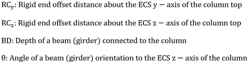
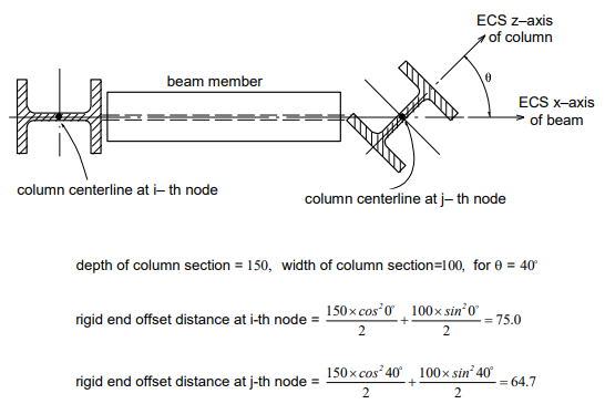
The rigid end offset distance of a beam (girder) member at a column is based on the depth and width of the column member at the beam-end and calculated as follows: Formula for calculating rigid end offset distance in each direction (See Figure 12)

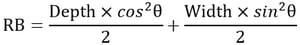
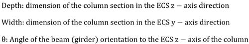
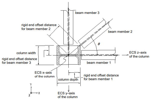
Figure 12. Rigid and Offset Distances of Beam (Girder) Members Using “Panel Zone Effects”

Method for the rigid end offset distances at both ends of beams using "Beam End Offsets"

“Beam End Offsets” allows the user to specify rigid end offset distances using the following two methods.²

* Refer to “Model > Boundaries>Beam End Offsets of Online Manual.

1. Offset distances at both ends are specified in the X, Y, and Z-axis direction components in the GCS
2. Offset distances at both ends are specified in the ECS x-direction

The first method is generally used to specify eccentricities at connections. In this case, the length between the end offsets is used to calculate element stiffness, distributed load, and self-weight. The locations for member force output and the end releases are also adjusted relative to the end offsets (See Figures 7 (b) & (c)).

The second method is used to specify eccentricities in the axial direction. It produces identical element stiffness, force output locations, and end release conditions to the case where “Panel Zone” with an offset factor, 1.0 is selected in Panel Zone Effects. However, the full length between two nodes is used for distributed loads, instead of the adjusted length.

Master and Slave Nodes (Rigid Link Function)

The rigid link function specified in Model>Boundaries > Rigid Link constrains geometric, relative movements of a structure. Geometric constraints of relative movements are established at a particular node to which one or more nodal degrees of freedom (d.o.f.) are subordinated. The particular reference node is called a Master Node, and the subordinated nodes are called Slave Nodes.

The rigid link function includes the following four connections:

1. Rigid Body Connection
2. Rigid Plane Connection
3. Rigid Translation Connection
4. Rigid Rotation Connection

Rigid Body Connection constrains the relative movements of the master node and slave nodes as if they are interconnected by a three-dimensional rigid body. In this case, relative nodal displacements are kept constant, and the geometric relationships for the displacements are expressed by the following equations:

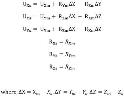
The subscripts, m, and s, in the above equations, represent a master node and slave nodes respectively. U_X, U_Y, and U_Z are displacements in the Global Coordinate System (GCS) X, Y, and Z directions respectively, and R_X, R_Y, and R_Z are rotations about the GCS X, Y, and Z-axes respectively. X_m, Y_m, and Z_m represent the coordinates of the master node, and X_s, Y_s, and Z_s represent the coordinates of a slave node. This feature may be applied to certain members whose stiffnesses are substantially larger than the remaining structural members such that their deformations can be ignored. It can be also used in the case of a stiffened plate to interconnect its plate and stiffener.

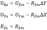
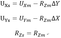
Rigid Plane Connection constrains the relative movements of the master node and slave nodes as if a planar rigid body parallel with the X-Y, Y-Z, or Z-X plane interconnects them. The distances between the nodes projected on the plane in question remain constant. The geometric relationships for the displacements are expressed by the following equations:

▶Rigid Plane Connection assigned to X-Y plane

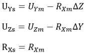
▶Rigid Plane Connection assigned to Y-Z plane

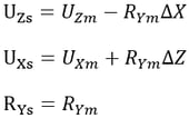
▶Rigid Plane Connection assigned to Z-X plane

This feature is generally used to model floor diaphragms whose relative in-plane displacements are negligible.

Rigid Translation Connection constrains relative translational movements of the master node and slave nodes in the X, Y, or Z-axis direction. The geometric relationships for the displacements are expressed by the following equations:

▶Displacement constraint in the X-axis direction

▶Displacement constraint in the Y-axis direction

▶Displacement constraint in the Z-axis direction

Rigid Rotation Connection constrains the relative rotational movements of the master node and slave nodes about the X, Y, or Z-axis. The geometric relationships for the displacements are expressed by the following equations:

▶Rotational constraint about the X-axis

▶Rotational constraint about the Y-axis

▶Rotational constraint about the Z-axis

The following illustrates an application of Rigid Plane Connection to a building floor diaphragm to help the user understand the concept of the rigid link feature.

When a building is subjected to a lateral load, the relative horizontal deformation at any point in the floor plane is generally negligible compared to that from other structural members such as columns, walls, and bracings. This rigid diaphragm action of the floor slab can be implemented by constraining all the relative in-plane displacements to behave as a unit. The movements consist of two in-plane translational displacements and one rotational displacement about the vertical direction.

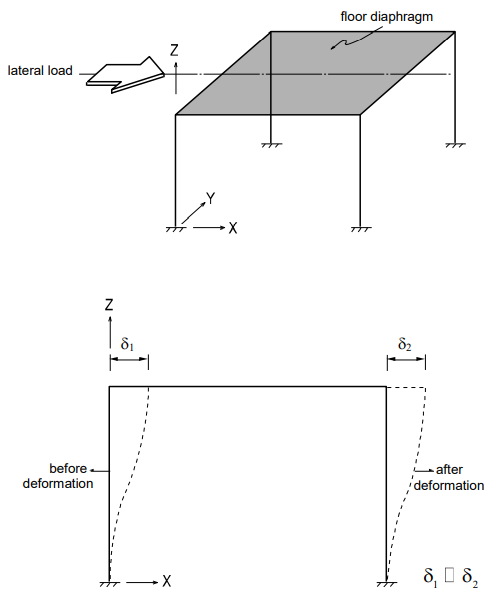
As illustrated in Figure 14, when a structure is subjected to a lateral load and the in-plane stiffness of the floor is significantly greater than the horizontal stiffness of the columns, the in-plane deformations of the floor can be ignored. Accordingly, the values of δ₁ and δ₂ may be considered equal.

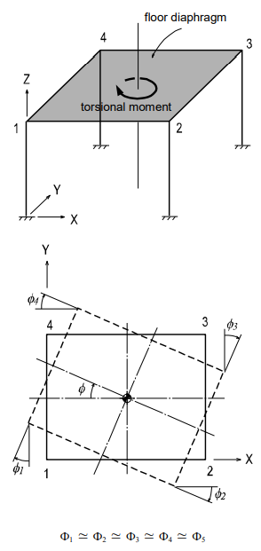
When a single-story structure, as illustrated in Figure 15, is subjected to a torsional moment about the vertical direction and the in-plane stiffness of the floor is significantly greater than the horizontal stiffness of the columns, the entire floor diaphragm will be rotated by ø, where, ø = ø₁= ø₂ = ø₃ = ø₄. Accordingly, the four degrees of freedom can be reduced to a single degree of freedom.

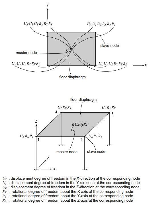
Figure 16 shows a process in which a total of 24 (6x4) degrees of freedom are compressed to 15 d.o.f. within the floor plane, considering its diaphragm actions.

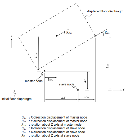
As illustrated in Figure 17, if translational and rotational displacements take place simultaneously in an infinitely stiff floor diaphragm due to a lateral load, the displacements of a point on the floor plane can be obtained by:

Reducing number of degrees of freedom by geometric constraints can significantly reduce the computational time for analysis. For instance, if a building structure is analyzed with the floors modeled as plate or plane stress elements, the number of nodes will increase substantially. Each additional node represents 3 additional degrees of freedom even if one considers d.o.f in lateral directions only. A large number of nodes in an analysis can result in excessive program execution time, or it may even surpass the program capacity. In general, solver time required is proportional to the number of degrees of freedom to the power of 3. It is, therefore, recommended that the number of degrees of freedom is minimized as long as the accuracy of the results is not compromised.

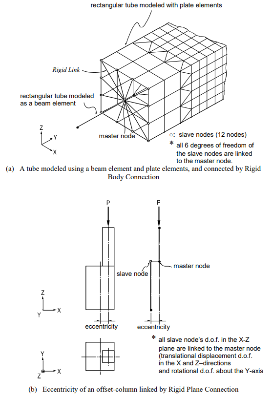
Figure 18 shows applications of Rigid Body Connection and Rigid Plane Connection. Figure 18 (a) illustrates an application of Rigid Link using Rigid Body Connection. Here a rectangular tube is modeled with plate elements in the region where a detailed review is required, beyond which a beam element represents the tube. Then, Rigid Body Connection joins the two regions.

Figure 18 (b) shows an application of Rigid Plane Connection for a column offset in a two-dimensional plane. Whenever a rigid link is used in a plane, geometric constraints must be assigned to two translational displacement components and one rotational component about the perpendicular axis to the plane.

If a structural analysis model includes geometric constraints and is used for dynamic analysis, the location of the master node must coincide with the mass center of all the masses pertaining to the slave nodes. This condition also applies to the masses converted from self-weights.

Specified Displacements of Supports

“Specified Displacements of Supports” is used to examine structural behaviors under the condition where displacements for restrained degrees of freedom are known in advance. It is also commonly referred to as “Forced Displacements”.

* Refer to “Load > Specified Displacements of Supports" of Online Manual.

In practice, this function is effectively used in the following cases:

• Detail safety assessment of an existing building, which has experienced post-construction deformations.
• Detail analyses of specific parts of the main structure. Displacements obtained from the analysis of a total structure form the basis of boundary conditions for analyzing specific parts.
• Analyses of existing buildings for foundation support settlements.
• Analyses of bridges reflecting support settlements

MIDAS/Gen allows you to define Specified Displacements of Supports by individual load cases. If Specified Displacements of Supports are assigned to unrestrained nodes, the program automatically restrains the corresponding degrees of freedom of the nodes. A separate data file is required if the analysis results of unrestrained degrees of freedom are desired.

Entering accurate values for Specified Displacements of Supports may become critical since structural behaviors are quite sensitive to even a slight variation. Thus, whenever possible, specifying all six degrees of freedom is recommended. In the case of analyzing an existing structure for safety evaluation, a deformed shape analysis may be required. However, it is typically not possible to measure in-situ rotational displacements. In such a case, only translational displacements are specified for an approximate analysis, but the resulting deformations must be reviewed against the deformations of the total structure.

When the displacements are obtained from the initial analysis of a total structure and subsequently used for a detailed analysis of a particular part of the structure, all 6 nodal degrees of freedom must be specified at the boundaries. In addition, all the loads present in the detailed model must be specified.

Specified Displacements generally follow the GCS unless NCS are previously defined at the corresponding nodes.

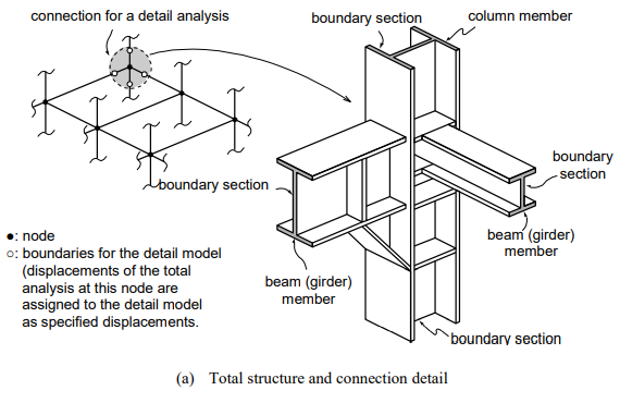
Figure 19 illustrates a procedure for analyzing a beam-corner column connection in detail.

1. As shown on the left-hand side of Figure 19 (a), an initial analysis is performed for the entire structure, from which the displacements at the connection nodes and boundaries are extracted for a detailed analysis.
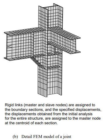
2. A total of 24 displacement components (6 d.o.f. per node) extracted from the 4 boundary nodes are assigned to the model, as shown to the right of Figure 19 (a). A master node is created at the centroid of each boundary section, and slave nodes are created and connected to the master node by Rigid Link at each section. The nodal displacements at the boundary sections from the analysis results of the entire structure are applied to the master nodes. Boundary sections should be located as far as possible from the zone of interest for detail analysis in order to reduce errors due to the effects of using Rigid Link.²
3. All the loads (applied to the entire structure model) that fall within the range of the detailed analysis model are entered for subsequent detail analysis.
4.