 Banner Title Products
What is Geometric Nonlinear Analysis?
When a structure is analyzed for linear elastic behaviors, the analysis is carried out on the premise that a proportional relationship exists between loads and displacements. This assumes a linear material stress-strain relationship and small geometric displacements.
The assumption of linear behaviors is valid in most structures. However, nonlinear analysis is necessary when stresses are excessive, or large displacements exist in the structure. Construction stage analyses for suspension and cable-stayed bridges are some of large displacement structure examples.
Nonlinear analysis can be classified into 3 main categories.
First, material nonlinear behaviors are encountered when relatively big loadings are applied to a structure thereby resulting in high stresses in the range of nonlinear stress-strain relationship. The relationship, which is typically represented as in Figure 1, widely varies with loading methods and material properties.
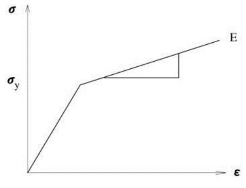
Figure 1. Stress-Strain Relationship Used for Material Nonlinearity
Second, a geometric nonlinear analysis is carried out when a structure undergoes large displacements and the change of its geometric shape renders a nonlinear displacement-strain relationship.
The geometric nonlinearity may exist even in the state of linear material behaviors. Cable structures such as suspension bridges are analyzed for geometric nonlinearity. A geometric nonlinear analysis must be carried out if a structure exhibits a significant change of its shape under applied loads such that the resulting large displacements change the coordinates of the structure or additional loads like moments are induced (See Figure 2).
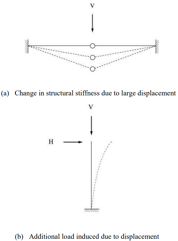
Figure 2. Structural System Requiring Geometric Nonlinear Analyses
Third, boundary nonlinearity of a load-displacement relationship can occur in a structure where boundary conditions change with its structural deformations due to external loads.
An example of boundary nonlinearity would be compression-only boundary conditions of a structure in contact with soil foundation.
MIDAS/Gen contains such nonlinear analysis functions as boundary nonlinear analysis using nonlinear elements (compression/tension-only elements) and large displacement geometric nonlinear analysis.
You can download the full content, after filling out the form at the end of this page.
Geometric Nonlinear Analysis
Small displacement (εij) used in linear analysis is given below under the assumption of small rotation.
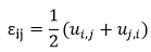
“u” represents displacement and “,” represents the differentiation of the first subscript coordinate. When a large displacement occurs as shown in Figure 3, the structural deformation cannot be expressed with small strain any longer. Large displacement can be divided into rotational and non-rotational components as per the equations below. F, R and U represent deformation tensor, rotation tensor and stretch tensor respectively. U determines the deformation of a real structure.
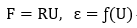
Accurate strain can be calculated from the above equations after eliminating the rotational component. When the magnitude of rotation is large, an accurate deformation displacement relationship cannot be found initially. That is, geometric nonlinearity is introduced because the deformations change according to the displacements calculated from the linear analysis.
Figure 3. Geometric Nonlinearity due to Large Displacement
MIDAS/Gen uses the co-rotational method for geometric nonlinear analysis, and its basic concept and analysis algorithm are as follows: This method considers geometric nonlinearity by using the strain in the Co-rotational coordinate system, which moves with the rotation of the element being deformed. The deformation-displacement relationship in the Co-rotational coordinate system can be expressed as a matrix equation,  , and the deformation displacement relationship matrix used in linear analysis can be applied. That is, the element’s stability and converging ability of linear analysis are maintained even geometric nonlinearity concepts are introduced. Maintaining such superior characteristics is most advantageous for nonlinear analysis.
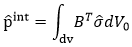
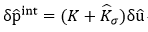
Displacement in the Co-rotational coordinate system is calculated by the equation, û = {e1, e2, e3, e1, e2, e3} and the infinitesimal displacement δû is “linearized” and then expressed as δû = Tδu . In the case of a linear elastic problem in the Co-rotational coordinate system, the internal element force
![]() is obtained from
is obtained from
where,
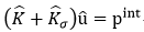
![]() is the stress expressed in the Co-rotational coordinate system, and the increment of the above equation becomes
is the stress expressed in the Co-rotational coordinate system, and the increment of the above equation becomes
![]()
is the geometric stiffness matrix or initial stress stiffness matrix. The following nonlinear equilibrium equation can be obtained using the equilibrium relationship between the internal and external forces, pext-pint=0.
Newton-Raphson and Arc-length methods are used for finding solutions to the nonlinear equilibrium equations. The Newton-Raphson method, which is a load control method, is used for typical analyses. For those problems such as Snap through or Snap-back, the Arc-length method is used.
MIDAS/Gen permits the use of truss, beam, and plate elements for geometric nonlinear analyses. If other types of elements are used, the stiffness is considered, but not the geometric nonlinearity.
Newton-Raphson Iteration Method
In the geometric nonlinear analysis of a structure being subjected to external loads, the geometric stiffness is expressed as a function of the displacement, which is then affected by the geometric stiffness again. The process requires repetitive analyses. The Newton-Raphson method is a widely used method, which calculates the displacement in equilibrium with the given external load as shown in Figure 4. The stiffness matrix is rearranged in each cycle of repetitive calculations to satisfy equilibrium with the load given in the equilibrium equation of load-displacement. A solution within the allowable tolerance is obtained using the stiffness matrices through the process of iteration.
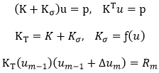
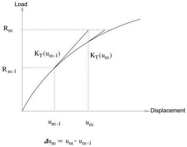
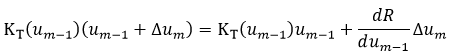
The process of analysis is illustrated in the above diagram. Once Δum is calculated, the displacement is adjusted by um = um-1 + Δum . To proceed to the next iterative step, a new tangential stiffness KT(um) and the unbalanced load Rm+1 - Rm are calculated, and the adjusted displacement um+1 is obtained.
The iterative process is continued until the magnitude of an increment in displacement, energy or load in a step is within the convergence limit.
Arc-Length Iteration Method
In a general iterative process, the calculated value for a displacement increment can be excessive if the load-displacement curve is close to horizontal. If the load increment remains constant, the resulting displacement can be quite excessive. The Arc-length method resolves such problems, and Snap-through behaviors can be analyzed similar to using the displacement control method. Also, the Arclength method can analyze even the Snap-back behaviors, which the displacement control method cannot analyze (See Figure 5(b)).
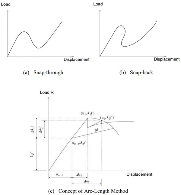
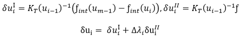
In the Arc-length method, the norm of incremental displacements is restrained to a pre-defined value. The magnitude of the increment is applied while remaining unchanged in the iterative process, but it is not fixed at the starting time of increments. The following process is observed in order to determine the magnitude of the increment: (Figure 5(c)) We define the external force vector at the beginning of increments as Rm-1 and the increment of external force vector as Δλiƒ.
The unit load ƒ is multiplied by the load coefficient Δλi and changed at every step of iteration.
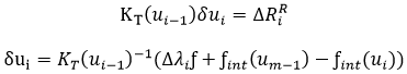 The solutions to the above equations can be divided into the following two parts, and the incremental displacement can be found below.
MIDAS/Gen finds the load coefficient Δλi by using the spherical path whose constraint condition equation is as follows:
Δl represents the displacement length to be restrained, and the equation Δui = Δui-1+δui is substituted into the above equation to calculate the load coefficient Δλi as below.
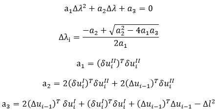
Generally, two solutions exist from the above equations. In the case of complex number solutions, linear equivalent solutions of the spherical path method are used. In order to determine which one of the real number solutions is to be used, the angle θ formed by the incremental displacement vectors of the preceding and present steps of iteration is calculated and used as per the equation below.
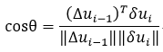
If the solutions contain one negative and one positive values, the positive value is selected. If both solutions produce acute angles, the solution close to the linear solution Δλi = -a3/a2 is used.
P-Delta Analysis
The P-Delta analysis option in MIDAS/Gen is a type of Geometric nonlinearity, which accounts for secondary structural behavior when axial and transverse loads are simultaneously applied to beam or wall elements. The P-Delta effect is more profound in tall building structures where high vertical axial forces act upon the laterally displaced structures caused by high lateral forces.
Virtually all design codes such as ACI 318 and AISC-LRFD specify that the P-Delta effect be included in structural analyses to account for more realistic member forces.
The P-Delta analysis feature in MIDAS/Gen is founded on the concept of the numerical analysis method adopted for Buckling analysis. Linear static analysis is performed first for a given loading condition and then a new geometric stiffness matrix is formulated based on the member forces or stresses obtained from the first analysis. The geometric stiffness matrix is thus repeatedly modified and used to perform subsequent static analyses until the given convergence conditions are satisfied.
As shown in Figure 6, static loading conditions are also required to consider the P-Delta effect for dynamic analyses.
The concept of the P-Delta analysis used in MIDAS/Gen is shown below.
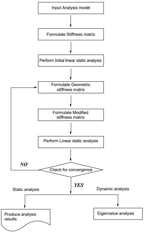
Figure 6. Flow Chart for P-Delta Analysis in MIDAS/GEN
When a lateral load acts upon a column member thereby resulting in moments and shear forces in the member, an additional tension force reduces the member forces whereas an additional compression force increases the member forces. Accordingly, tension forces acting on column members subjected to lateral loads increase the stiffness pertaining to lateral behaviors while compression forces have an opposite effect on the column members.
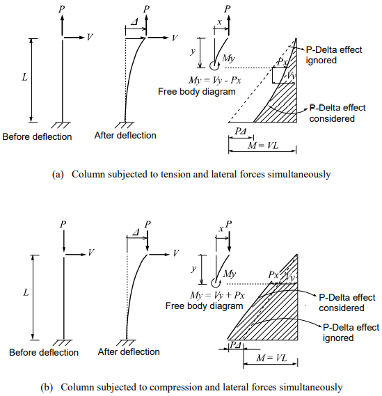
Figure 7. Column Behaviors due to P-Delta Effects
If the P-Delta effect is ignored, the column moment due to the lateral load alone varies from M=0 at the top to M=VL at the base. The additional tension and compression forces produce negative and positive P-Delta moments respectively. The effects are tantamount to an increase or decrease in the lateral stiffness of the column member depending on whether or not the additional axial force is tension or compression.
Accordingly, the lateral displacement can be expressed as a function of lateral and axial forces.
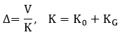
K0 here represents the intrinsic lateral stiffness of the column and KG represents the effect of change (increase/decrease) in stiffness due to axial forces. Formulation of geometric stiffness matrices for truss, beam and plate elements can be found in Buckling Analysis.
The P-Delta analysis can be summarized as follows:
1st Step Analysis

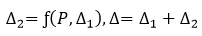
2nd Step Analysis
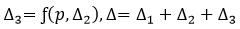
4th Step Analysis
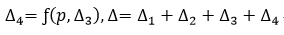
Nth Step Analysis

After obtaining Δ1 from the 1st step analysis, the geometric stiffness matrix due to the axial force is found, which is then added to the initial stiffness matrix to form a new stiffness matrix. This new stiffness matrix is now used to calculate Δ2 reflecting P-Delta effects, and the convergence conditions are checked. The convergence conditions are defined in “P-Delta Analysis Control”, which are Maximum Number of Iteration and Displacement Tolerance. The above steps are repeated until the convergence requirements are satisfied.
Note that the P-Delta analysis feature in MIDAS/Gen produces very accurate results when lateral displacements are relatively small (within the elastic limit).
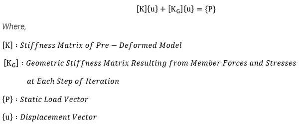
The static equilibrium equation for P-Delta analysis used in MIDAS/Gen can be expressed as
P-Delta analysis in MIDAS/Gen premises on the following:
-
Geometric stiffness matrices to consider P-Delta effects can be formulated only for truss, beam and wall elements.
-
Lateral deflections (bending and shear deformations) of beam elements are considered only for “Large-Stress Effect” due to axial forces.
-
P-Delta analysis is valid within the elastic limit.
In general, it is recommended that P-Delta analysis be carried out at the final stage of structural design since it is a time-consuming process in terms of computational time.
Analysis Using Nonlinear Elements
Nonlinear analysis in MIDAS/Gen is applied to a static analysis of a linear structure in which some nonlinear elements are included. The nonlinear elements that can be used in such a case include tension-only truss element, hook element, cable element, compression-only truss element, gap element and tension/compression-only of Elastic Link. The static equilibrium equation of a structural system using such nonlinear elements can be written as
<Eq. 1>
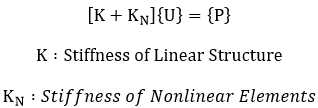
The equilibrium equation containing the nonlinear stiffness, KN, in <Eq. 1> can be solved by the following two methods:
The first method seeks the solution to the equation by modifying the loading term without changing the stiffness term. The analysis is carried out by the following procedure:
If we apply the stiffness of nonlinear elements at the linear state to both sides of the equation, and move the stiffness of nonlinear elements to the loading term, <Eq. 2> can be derived.
<Eq. 2>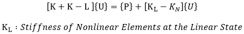
In <Eq. 2>, the linear stiffness of the structure and the stiffness of nonlinear elements at the linear state always remain unchanged. Therefore, static analysis of a structure containing nonlinear elements can be accomplished by repeatedly modifying the loading term on the right side of the equation without having to repeatedly recompose the global stiffness or decompose the matrix. Not only does this method readily perform nonlinear analysis, but also reducing analysis time is an advantage without the reformation process of stiffness matrices where multiple loading cases exist.
The second method seeks the solution to the equation by iteratively reassembling the stiffness matrix of the structure without varying the loading term following the procedure below.
A static analysis is performed by initially assuming the stiffness of nonlinear elements in <Eq. 1> . Using the results of the first static analysis, the stiffness of nonlinear elements is obtained, which is then added to the stiffness of the linear structure to form the global stiffness. The new stiffness is then applied to carry out another round of static analysis, and this procedure is repeated until the solution is found. This method renders separate analyses for different loading conditions as the stiffness matrices for nonlinear elements vary with the loading conditions.
The above two methods result in different levels of convergence depending on the types of structures. The first method is generally effective in analyzing a structure that contains tension-only bracings, which are quite often encountered in building structures. However, the second method can be effective for analyzing a structure with soil boundary conditions containing compression-only elements.
Stiffness of Nonlinear Elements (KN)
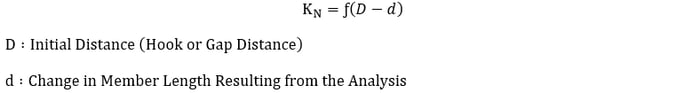
MIDAS/Gen calculates the stiffness of nonlinear elements by using displacements and member forces resulting from the analysis. The nonlinear stiffness of Truss, Hook and Gap types is determined on the basis of displacements at both ends and the hook or gap distance. The nonlinear stiffness of cable elements is obtained from the resulting tension forces.
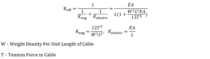
The nonlinear stiffness of tension/compression–only elements such as Truss, Hook and Gap types can be determined by <Eq. 3>. Whereas, stiffness changes for tension-only cable elements need to be considered according to the changes of tension forces in the members. The nonlinear stiffness is calculated by determining the effective stiffness, which is expressed in <Eq. 4>.
<Eq. 3>
 <Eq. 4>
Since the nonlinear elements used in MIDAS/Gen do not reflect the large displacement effect and material nonlinearity, some limitations for applications are noted below.
- Material nonlinearity is not considered.
- Nonlinearity for large displacements is not considered.
- Instability due to loadings may occur in a structure, which is solely composed of nonlinear elements. The use of nodes composed of only nonlinear elements are not allowed.
- Element stiffness changes with changing displacements and member forces due to applied loadings. Therefore, linear superposition of the results from individual loading cases are prohibited.
- In the case of a dynamic analysis for a structure, which includes nonlinear elements, the stiffness at the linear state is utilized.
The analysis procedure for using nonlinear elements is as follows:
- Using the linear stiffness of the structure and the stiffness of nonlinear elements at the linear state, formulate the global stiffness matrix and load vector.
- Using the global stiffness matrix and load vector, perform a static analysis to obtain displacements and member forces.
- Re-formulate the global stiffness matrix and load vector.
- If method 1 is used, where the analysis is performed without changing the stiffness term while varying the loading term, the nonlinear stiffness is computed by using the displacements and member forces obtained in Step 2, which is then used to reformulate the loading term. If method 2 is used, where the analysis is performed with changing the stiffness term, the stiffness of nonlinear elements is computed first by using the resulting displacements and member forces, which is then used to determine the global stiffness matrix.
- Repeat steps 2 and 3 until the convergence requirements are satisfied.